Learn · Updated
How Do Music Visualisers Work?
Short answer: Music visualisers work by repeatedly taking a short window of audio samples, measuring its amplitude and, using a Fast Fourier Transform (FFT), its frequency content, then mapping those values to visual parameters and drawing a new frame.
Music visualisers work by analysing short slices of audio and mapping the measurements to graphics, many times per second. Underneath the variety of styles, almost all of them use the same few building blocks.
1. Digital audio is a list of samples
A digital audio file stores sound as a sequence of numbers called samples, each representing the air pressure at one instant. CD-quality audio uses 44,100 samples per second per channel; 48,000 is common for video.
A visualiser running at 60 frames per second has about 735 new samples per channel to work with for each frame at 44.1 kHz. In practice it analyses a slightly larger, overlapping window, often 1,024 or 2,048 samples.
2. Amplitude: how loud it is
The simplest measurement is amplitude. Drawing the raw samples gives a waveform. Summarising a window as a single loudness value gives the level used to pulse an object or drive a VU meter. Visualisers usually use RMS (root mean square), which tracks perceived loudness better than the peak value.
3. Frequency: what the sound contains
To show bass, mids and treble separately, visualisers convert the window from the time domain to the frequency domain with a Fast Fourier Transform (FFT). The FFT outputs bins, each holding the energy in a narrow frequency range.
The width of each bin is the sample rate divided by the FFT size. At 44.1 kHz with an FFT size of 2,048, each bin is about 21.5 Hz wide, giving 1,024 usable bins up to 22,050 Hz.
Because human hearing is roughly logarithmic, with each octave doubling in frequency, spectrum visualisers rarely show bins linearly. They group bins into logarithmic or octave bands, so the bass is not squeezed into the first few pixels. Accurate analysers such as audioMotion offer fractional-octave bands and perceptual scales like Bark and Mel.
| Range | Approximate frequencies | Typical sources |
|---|---|---|
| Sub-bass | 20–60 Hz | Kick drum body, 808s |
| Bass | 60–250 Hz | Bass guitar, synth bass |
| Mids | 250 Hz–4 kHz | Vocals, guitars, snares |
| Highs | 4–20 kHz | Cymbals, hi-hats, “air” |
4. Smoothing and scaling
Raw FFT values jump around from frame to frame. Visualisers apply:
- Temporal smoothing: averaging with previous frames so bars rise quickly and fall gradually.
- Decibel scaling: converting energy to a logarithmic dB scale, closer to how loudness is heard.
- Normalisation or gain control: adjusting so quiet and loud tracks both fill the display.
In the browser, the Web Audio API’s AnalyserNode provides FFT data with built-in smoothing (its smoothingTimeConstant defaults to 0.8) and dB range settings.
5. Beat and onset detection
Many visuals respond to events, not just levels: a cut on each kick drum or a flash on each snare. Simple beat detection compares the current energy in a band with its recent average and triggers when it jumps above a threshold. More robust approaches use spectral flux, the sum of increases in energy across all bins, to find note onsets. Some tools also estimate tempo (BPM) so effects can run in time even between detected beats.
Higher-level features, such as spectral centroid (brightness), chroma (pitch class) or stem separation in AI tools like Neural Frames, allow visuals to follow specific musical qualities. JavaScript libraries such as Meyda compute these.
6. Mapping to visuals
Finally, analysis values are mapped to visual parameters:
- Literal mappings: bar heights equal band levels; the line follows the waveform. This is how spectrum and waveform visualisers work.
- Expressive mappings: bass level scales a 3D object, treble shifts colour, beats trigger camera cuts. This is the core of audio-reactive and generative visuals.
- Preset equations: in MilkDrop-style visualisers, presets read bass, mid and treble values inside per-frame and per-pixel equations.
Real-time vs offline rendering
A real-time visualiser must analyse and draw each frame within a few milliseconds, so it uses the GPU and limits complexity. An offline video maker can take as long as needed per frame, and because it has the whole file in advance, it can look ahead, for example to anticipate a drop. That is why rendered videos can be smoother and more detailed than live visuals on the same machine.
Next: Waveform vs spectrum visualisers or How audio-reactive visuals work.
Frequently asked questions
What is FFT in a music visualiser?
FFT (Fast Fourier Transform) is an algorithm that converts a short window of audio samples into frequency bins, each representing the energy in a narrow frequency range. Visualisers group those bins into bars or bands.
Why do visualiser bars fall slowly after a loud sound?
Visualisers apply smoothing so values decay gradually instead of jumping each frame. Without it, bars flicker and are hard to read.
How do visualisers detect beats?
A common approach compares the current energy, often in the bass range, with its recent average. A sudden rise above a threshold is treated as a beat or onset. More advanced methods measure spectral flux, the frame-to-frame increase in energy across frequencies.